Experiment 7: Introduction to Reflection and Refraction

Purpose:  To study the effects of reflection and refraction as they apply to light hitting and traveling through a semicircular prism as seen below.

Equipment:

• Light Source 
• Semicircular Glass/Plastic Prism
• Circular Protractor

Experiment:

Tape the protractor to the desk oriented such that the light enters at 180 degrees and exits at 0 degrees.  The initial setup is with the light entering perpendicular to flat side of the prism and exiting the curved side.  The angle of incidence and the angle of refraction for the light ray in this configuration is 0 degrees.  Nothing will happen to the light ray as it enters the prism from the air or enters the air from the prism since the light beam is hitting normal to the surface.  This experiments covers a situation where the light will travl from low density to high density and then back to low density.  Rotate the prism 10 degrees and record the angle of the light traveling through the prism.  Continue to do this and record the values . 

Below is the data table with these values.

Θ1	Θ2	sin(Θ1)	sin(Θ2)
0	0	0	0
10	4	0.1736482	0.0697565
20	8	0.3420201	0.1391731
30	12	0.5	0.2079117
40	15	0.6427876	0.258819
45	17	0.7071068	0.2923717
50	19	0.7660444	0.3255682
60	24	0.8660254	0.4067366
70	30	0.9396926	0.5
80	37	0.9848078	0.601815

Part 2 uses the same materials, however the prism will be roatated such that the light will enter on the circular side and exit the flat side.  Locate the prism with the flat side perpendicular to the light source but on the opposite side.  Similar to the photo shown below.  As the light enters the prism it will pass striaght through without "bending" since the flat surface is normal to the light beam.  This experiment again shows light traveling from low density to high denisty and back to low density.  Rotate the prism 10 degrees, record the angle of the light beam and repeat. 

Below is the data tables with these values.

Θ3	Θ4	sin(Θ3)	sin(Θ4)
0	0	0	0
10	5	0.173648	0.087156
15	8	0.258819	0.139173
20	12	0.34202	0.207912
25	13	0.422618	0.224951
30	15	0.5	0.258819
35	20	0.573576	0.34202
40	26	0.642788	0.438371
44	44	0.694658	0.694658
45	N/A	N/A	N/A

Conclusion:

In Part 1, the light would bend further and further as the prism rotated further around.  Below is a plot of the graph of sin(Θ₁) vs sin(Θ₂).  The trendline is y = 1.9944x. 




In Part 2, the light would bend further and further as the prism rotated further around. Below is a plot of the graph of sin(Θ₃) vs sin(Θ₄).  The trendline is y = 1.3346x. 

Experiment 6: Electromagnetic Radiation Lab

Purpose:
To use a simple antenna to study the behavior of electromagnetic radiation.   

Equipment:

• Small Guage Straight Copper Wire
• (2) Meter Sticks
• Frequency Generator
• Oscilloscope
• BNC Connector 

Experiment:

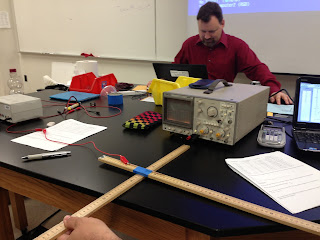
Create a transmitter by attaching the copper wire to a meter stick with masking tape and connect one end to the frequency generator.  Create a receiver by pluggin the BNC connector into the oscilloscope (channel 1).  Use the frequency generator to create a frequency of 30 kHZ and turn the amplitude to its maximum.  Change the time/div setting on the oscilloscope to 0.1 ms and decrease the voltage/div until a signal in seen on the screen.  Measure and record the peak to peak amplitude of the EM wave and record them for several trials. 

Below is the data table of these values.

Distance (m)	# of Divisions Peak to Peak	Vertical Scale (mV)	Peak to Peak Amplitude (mV)
0.5	3.3	10.0	5.5	55
0.1	3.2	10.0	5.0	50
0.2	3.2	10.0	4.0	40
0.2	3.2	5.0	6.4	32
0.3	3.2	5.0	5.2	26
0.3	3.2	5.0	4.8	24
0.4	3.2	5.0	4.2	21
0.4	3.2	5.0	4.0	20
0.5	3.2	5.0	3.2	16
0.5	3.2	5.0	2.8	14
0.6	3.2	5.0	2.6	13
0.6	3.2	5.0	2.4	12

Conclusion:

The data plot of peak to peak amplitude as a function of distance is shown below.  The graph appears to take on an inversely proportionate shape. 

The trendlines of A/r and A/r^2 are included on the graph.  The A/x function fits the data better than the A/r^2 does, however, still is not a great fit.  The A/r^n function that is also included fits the best.  The data does not fit the A/r function, what we would expect if it were a point charge, because the tansmitter is linear perpendicular to the receiver.  Therefore, we must take each dx and consider that instead of a single point source. 

Experiment 5: Introduction to Sound

Purpose:
To understand the shapes and characteristics of sound waves. 

Equipment:

• Lab Pro
• Microphone

Experiment:

Using logger pro, collect data while someone says, "AHHHHHH" into the microphone.  Answer the following questions about the graph that is produced:

1)     Would you say this is a periodic wave?  Support your answer with characteristics.

2)     How many waves are shown in this sample?  Explain how you determined this number.

3)     Relate how long the probe collected data to something in your everyday experience. For example: “Lunch passes by at a snails pace.” Or “Physics class flies by as fast as a jet by the window.”

4)     What is the period of these waves?  Explain how you determined the period.

5)    What is the frequency of these waves?  Explain how you determined the frequency.

6)     Calculate the wavelength assuming the speed of sound to be 340 m/s. Relate the length of the sound wave to something in the class room.

7)     What is the amplitude of these waves?  Explain how you determined amplitude.

8)     What would be different about the graph if the sample were 10 times as long? How would your answers for the questions a-g change? Explain your thinking. Change the sample rate and test your ideas. Copy the graph and label it #1h.

Have someone else speak into the microphone and compare and contrast the two graphs. 

Then use a tuning fork to produce a graph and compare and contrast that graph against the human graphs. 

What would you expect if the tuning fork wasn't as loud as the first time?

Conclusion:

Part A:

1)      This wave is periodic since it repeats similar to a sinusoidal wave. 

2)      5.4 waves are in this sample. 

3)      The data was collected over 0.03 seconds which is faster than you blink.

4)      The period of the wave is 0.0056 seconds.  We determined this by dividing the sample time (0.03) by the number of waves (5.4).

5)      The frequency is 180 Hz.  We determined this by 1/T and confirmed it by extrapolating 5.4 waves in .03 seconds and looked at how many waves in one second (frequency).

6)      The wavelength equals velocity divided by the frequency.  (340m/s) / (180 s^-1) = 1.89m.  This is about the length of a desk. 

7)      The amplitude is 1.8 units.  We determined this from the graph.

8)      Everything would be the same except you would have more waves in the sample. 

 

Part B:

The second wave sampling was not as regular as the first.  There are 3.5 waves in the sample which is 0.03 seconds.  The period is 0.0086 seconds.  The frequency of the wave is 116 Hz.  The wavelength is 2.93 m.  The amplitude is 0.75 units. 

Part C:

The tuning fork produces a much more uniform sound wave compared to the human waves.  There are 15 waves in the sample of 0.03 seconds.  The period is 0.0020 seconds.  The frequency of the wave is 500 Hz.  The wavelength is 0.68 m.  The amplitude is 0.23 units. 

Part D:

 

Only the amplitude of the wave changed (decreased) while the other data remained the same.  We changed the impact surface to a softer material (skin/pants vs rubber shoe sole) which resulted in a softer wave. 

Experiment 4: Standing Waves

Purpose:
To understand the characteristics of standing waves when in resonance and driven by an outside source. 

Equipment:

• String (2 meters)
• Pulley
• Mechanical Vibrator
• Function Generator
• Counterweight (50 g and 200 g)
• 2 meter Stick
• Various Lab Components



Experiment:

 

Attach a string to a ring stand on one side and over a pulley on the other. Place a 200 g counterweight on the end of the string. Connect the function generator to the mechanical vibrator and place it with the string passing just over the top closest to the end attached to the ring stand. Measure the effective distance (from mechanical vibrator to pulley) of the string. Adjust the function generator until the string oscillates in its fundamental mode. Record the number of nodes, the length between nodes, the wavelength, the frequency and voltage. Repeat for up to eight antinodes. Repeat entire experiment with 50 g counterwieght. 

 

 

0.00083	Mass of String (g)
2.495	Length of String (m)
0.0003327	Linear Density (kg/m)
1.800	Effective String Length (m)

 

Below is the data for the 200 g counterweight.

 

200 gram Counterweight
# of Antinode	Length Node to Node (m)	Frequency (Hz)	λ (m)	1/λ		Theoretical Speed
1	1.800	24	3.600	0.2778		86.40
2	0.910	44	1.800	0.5556		79.20
3	0.595	66	1.200	0.8333		79.20
4	0.450	88	0.900	1.1111		79.20
5	0.370	110	0.720	1.3889		79.20
6	0.310	131	0.600	1.6667		78.60
7	0.265	154	0.514	1.9444		79.20
8	0.225	177	0.450	2.2222		79.65
			Average Speed			80.08

Below is the data for the 50 g counterweight.

50 gram Counterweight
# of Antinode	Length Node to Node (m)	Frequency (Hz)	λ (m)	1/λ		Theoretical Speed
1	1.800	11	3.600	0.2778		39.60
2	0.900	22	1.800	0.5556		39.60
3	0.620	33	1.200	0.8333		39.60
4	0.470	44	0.900	1.1111		39.60
5	0.350	55	0.720	1.3889		39.60
6	0.315	66	0.600	1.6667		39.60
7	0.265	77	0.514	1.9444		39.60
8	0.225	88	0.450	2.2222		39.60
			Average Speed			39.60

Conclusion:

The theoretical value and experimental value ratios have a percent error of 1.6%. 

Experimental Values			Theoretical Values
78.771	Case 1 Speed (m/s)		80.08	Case 1 Speed (m/s)
39.600	Case 2 Speed (m/s)		39.600	Case 2 Speed (m/s)
1.989	Ratio Case 1/Case 2		2.022	Ratio Case 1/Case 2